In this tutorial you will get insights on the FinnGen health data supporting the glaucoma endpoint.

It usually takes 20–30 minutes to complete this tutorial, but we know not everyone has time to complete it in one seating. It's ok! This tutorial is designed to make it easy to start now and get back to it later.

Opening Risteys homepage

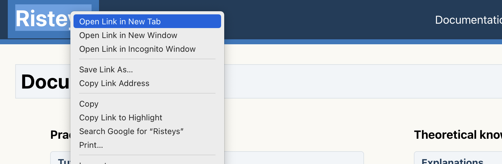
First, open Risteys homepage in a new tab so that we can easily navigate between this tutorial and there.

Go ahead and right-click on the big Risteys title at the top of this page, then select Open Link in New Tab:

You should now be able to quickly go back and forth between this tutorial page and Risteys homepage. Congrats, you are all set up for the next tutorial sections!

Searching for an endpoint

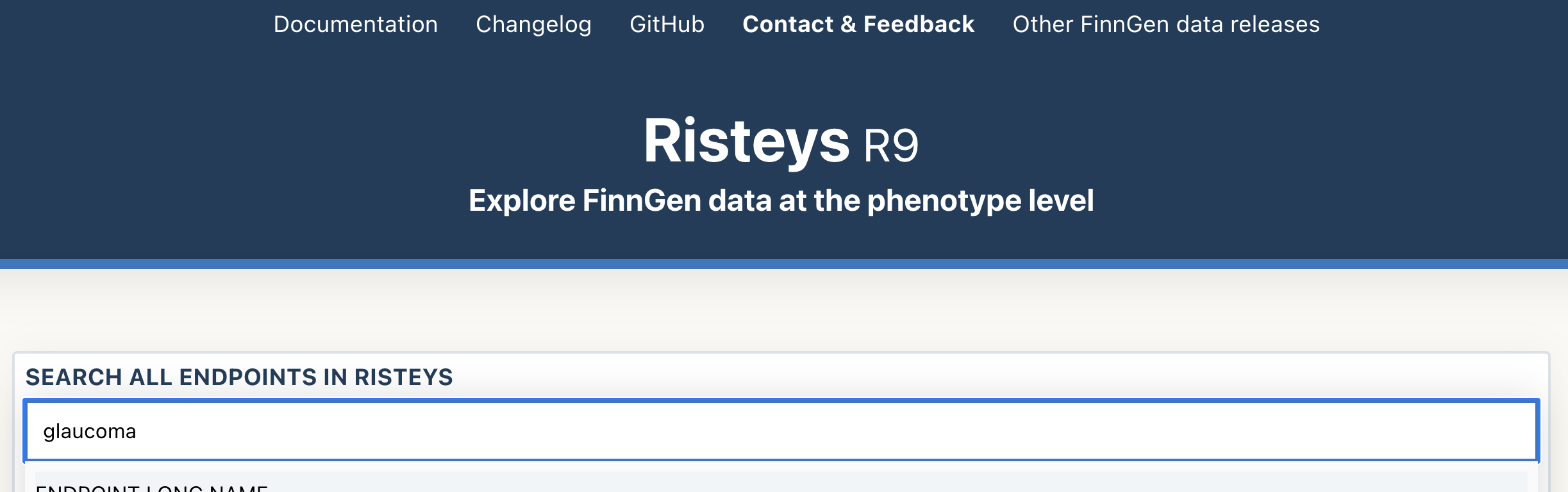
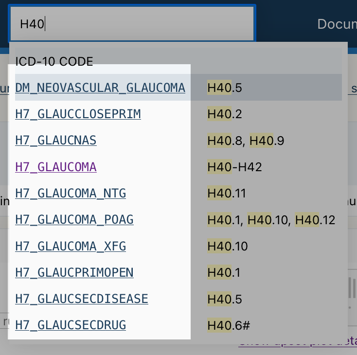
The Risteys homepage has a search bar. Click on it and type glaucoma:

Search results appear has you type, displaying endpoints matching the search query.

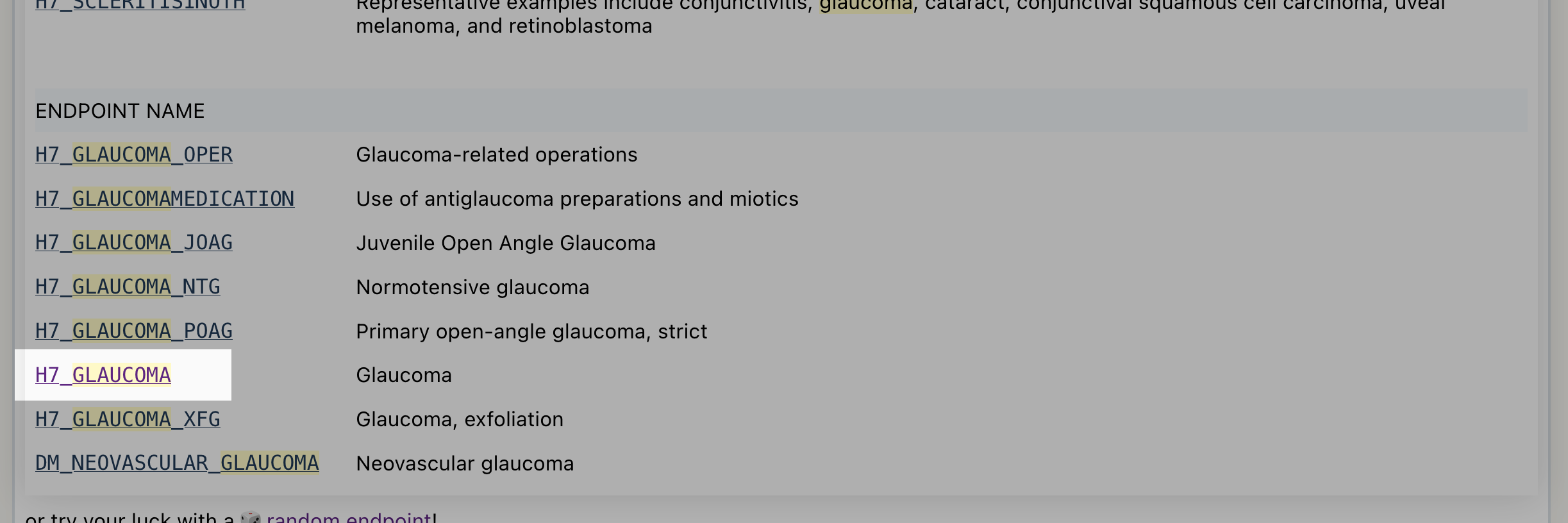
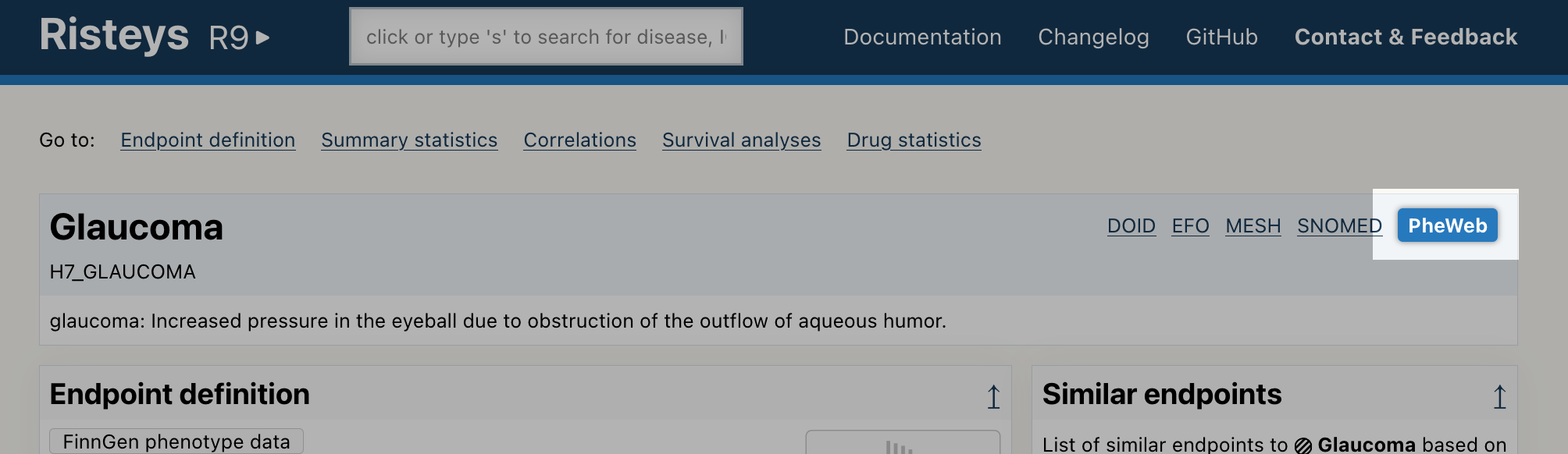
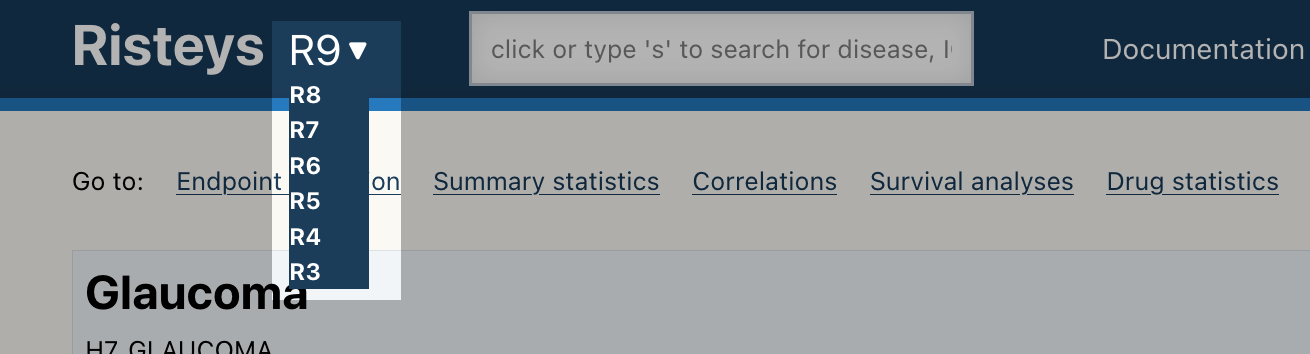
Scroll down the search results to locate the endpoint H7_GLAUCOMA:

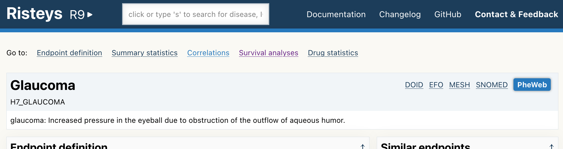
Click on the H7_GLAUCOMA link as shown above. It will take you to its endpoint page, it should look like this:

To make sure you are on the right page, check that you see a title Glaucoma near the top of the page, and the H7_GLAUCOMA code just below it. Like in the screenshot above.

You are now ready for the next section.

Checking how the endpoint is defined

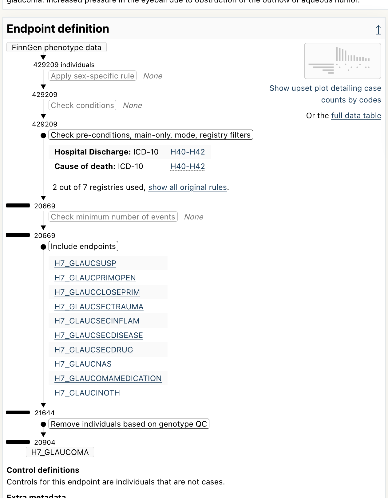
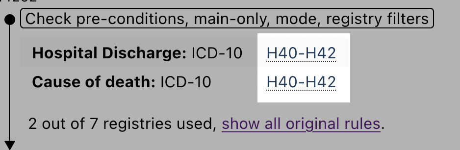
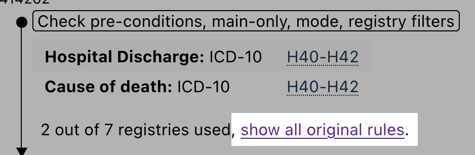
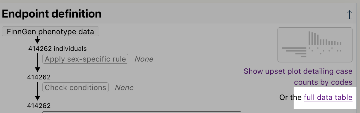
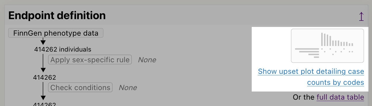
Now that you are on the glaucoma endpoint page, scroll down a bit to reveal the Endpoint definition section:

As we can see, this endpoint is defined using the ICD-10 code H40-H42, and it also include other endpoints.

Checking the upset plot for evidence of code usage

Click on the upset plot icon near the top of the page:

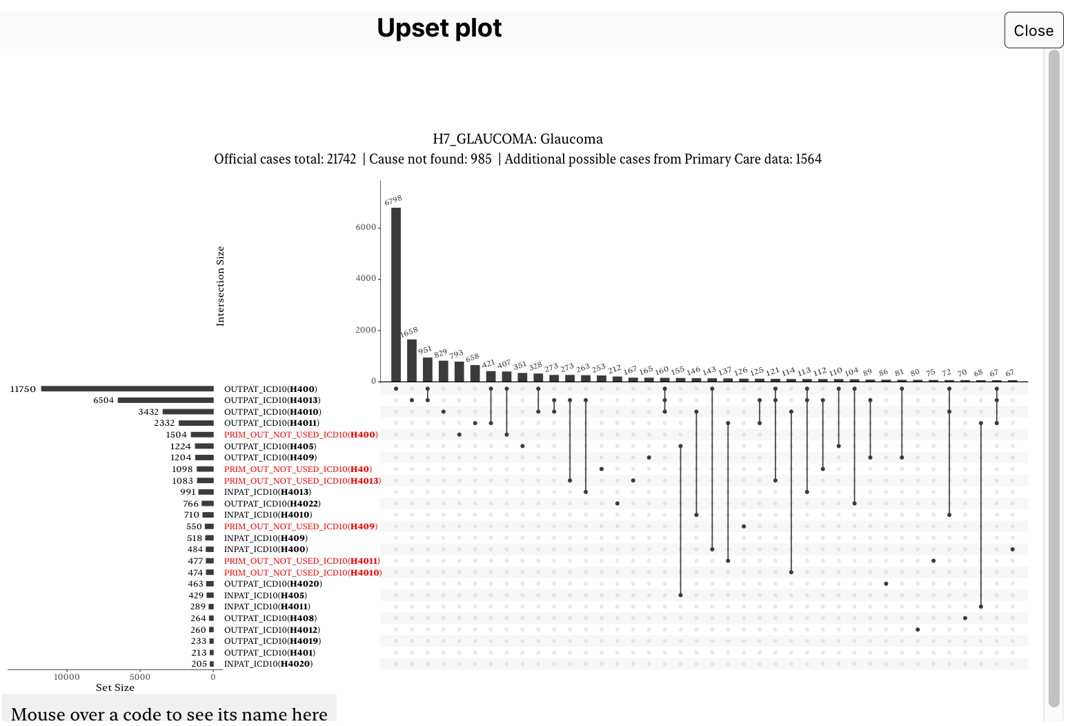
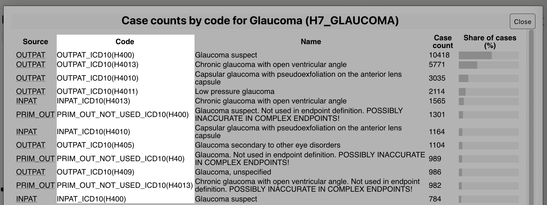
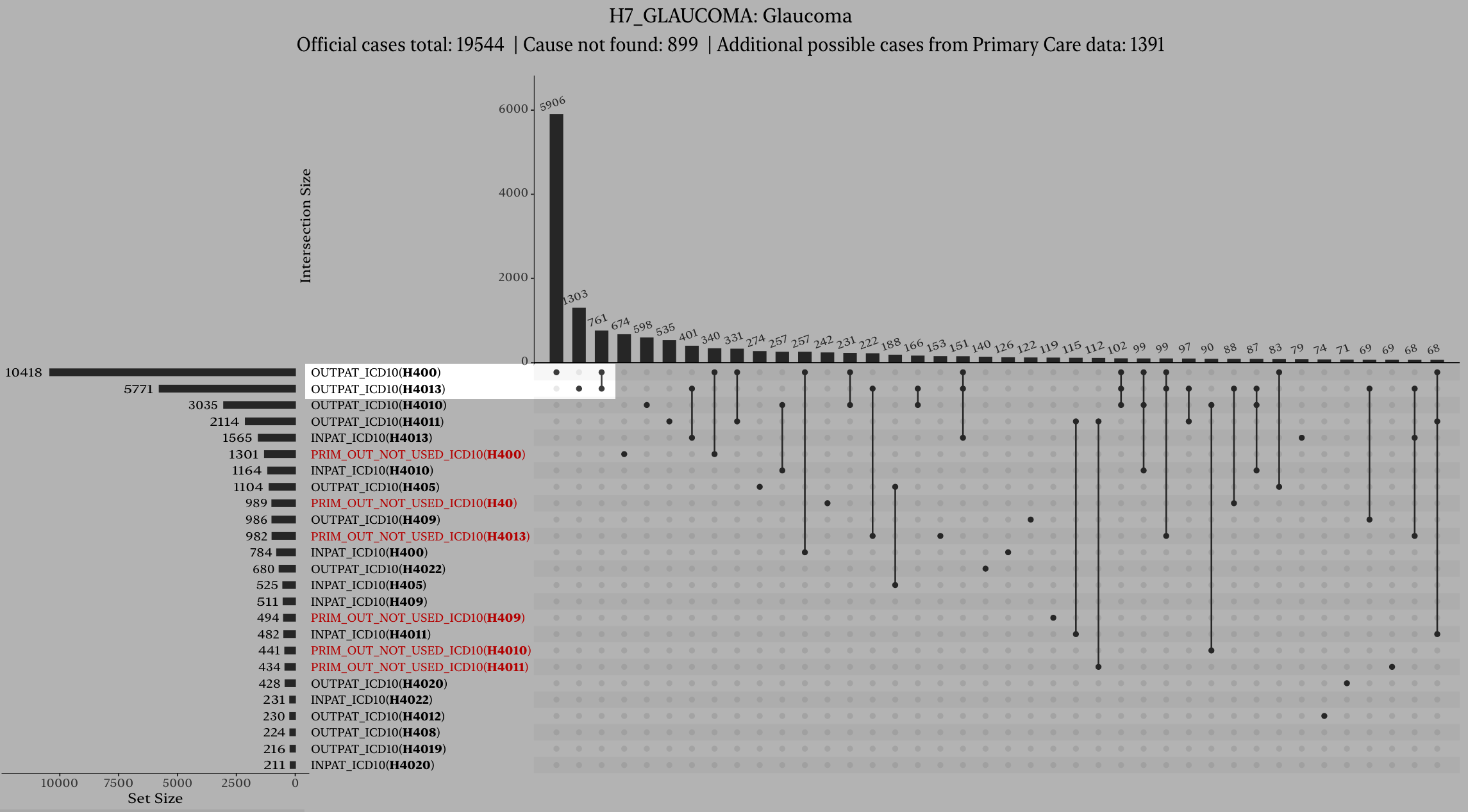
A window pops up with a list of code for that endpoint, and how the cases are distributed among these codes. It should look like this:

You can now close the upset plot by clicking on the Close button the top-right corner:

You are now back on the glaucoma endpoint page. You can continue to the next section.

Checking the summary statistics

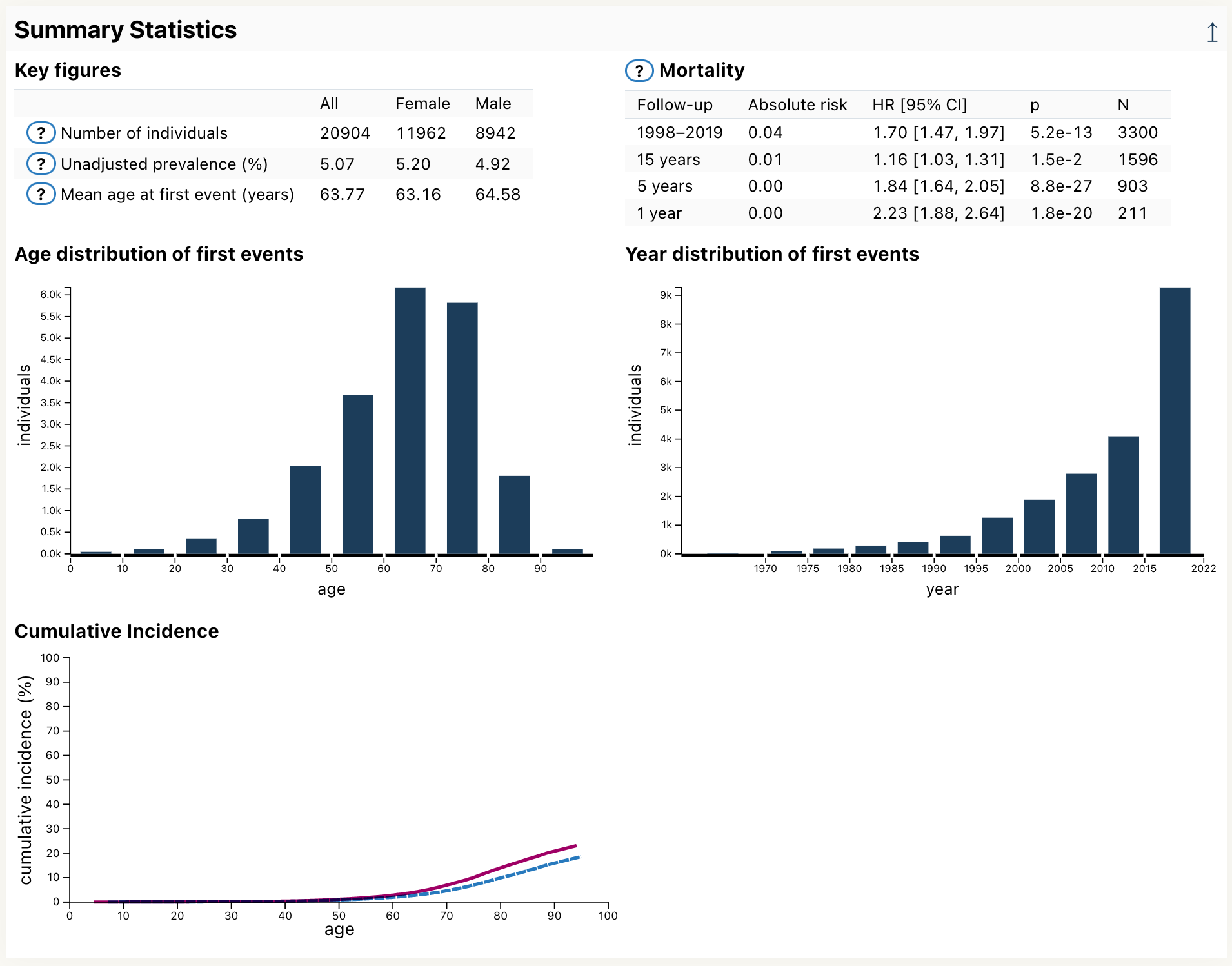
Scroll down the page until you see the section Summary Statistics:

Here you can different statistics for the glaucoma endpoint, such as:

• number of cases (20904)
• mean age at first event (63.77)

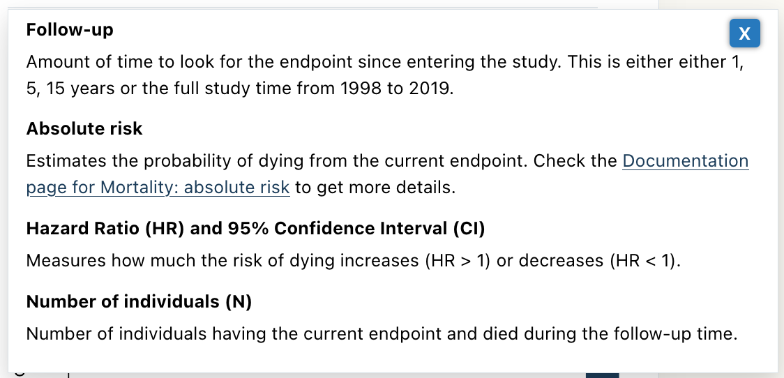
Click on the help icon next to Mortality:

A help panel pops in and provide explanations on how to interpret the mortality table:

Close this help panel by clicking on the X button on the top-right corner:

Notice there are other help buttons on the endpoint page. They explain different concepts and have the same open/close interaction.

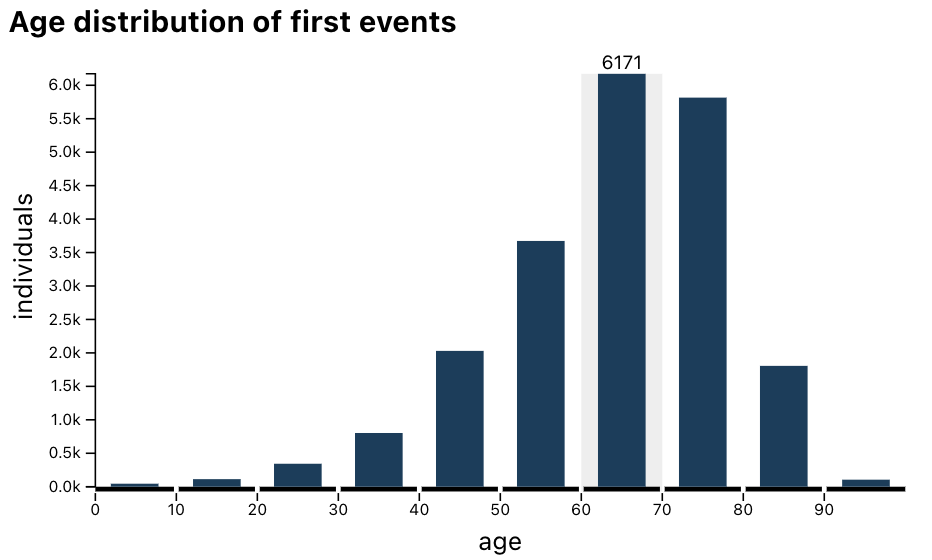
Hover over the 60–70 bin in the age distribution:

The plot now displays there are 6171 cases having a first event of glaucoma when they were between 60 and 70 years old.

The end

Congratulations! You have completed the Risteys tutorial.

You started by searching for the glaucoma endpoint, then checked how it is defined in FinnGen, and finally looked at its descriptive statistics.

Risteys has more to offer: feel free to look at other sections on the glaucoma endpoint page, check other endpoint pages, or browse the documentation below.

How to lookup endpoints that have a specific ICD-10-fi code?

1. Click on the search bar.
2. Enter the ICD-10-fi code of interest.

3. Click the endpoints in the search results. The matching ICD-10-fi are highlighted.

   

How to check which codes are used for a given endpoint?

There are 3 ways for checking which codes are used for an endpoint:

1. using the endpoint explainer
2. using the original rules
3. using the full data table of the upset plot

Using the endpoint explainer

1. Go to the endpoint page of your endpoint of interest.
2. Scroll down to Endpoint definition.
3. Locate the section Check pre-conditions, main-only, mode, registry filters.

4. Check the codes displayed in this section.

   

Using the original rules

1. Go to the endpoint page of your endpoint of interest.
2. Scroll down to Endpoint definition.
3. Locate the section Check pre-conditions, main-only, mode, registry filters.

4. Click show all original rules.

   

5. Read the rules as given in the original endpoint definitions.

   

Using the full data table of the upset plot

1. Go to the endpoint page of your endpoint of interest.
2. Scroll down to Endpoint definition.

3. Click on the link full data table.

   

4. Read the codes given to the endpoint cases in the Code column of the table.

   

Related documentation: How to check which combination of codes are the most common among endpoint cases?

How to check which combination of codes are the most common among endpoint cases?

1. Go to the endpoint page of your endpoint of interest.
2. Scroll down to Endpoint definition.

3. Click on the link Show upset plot detailing case counts by codes.

   

4. Read the left column for the codes, and the dot matrix for the combination of codes.

   

How to see the GWAS information and Manhattan plot for an endpoint?

1. Go to the endpoint page of your endpoint of interest.

2. Click the PheWeb button near the top-right of the page.

   

How to browse the data at a different data freeze? (e.g. FinnGen R5)

1. from the home page
2. from an endpoint page

From the home page

1. Go to the home page.
2. Hover over Other FinnGen data releases at the top of the home page.

3. Click on the data freeze version you want to browse.

   

From an endpoint page

1. Go to the endpoint page of your endpoint of interest.
2. At the top of the page, click on the arrow next to the current data freeze version.

3. Click on the data freeze version you want to browse.

   

How to find related endpoints to the one I am looking at?

There are two ways to accomplish this:

1. using the Similar endpoints feature
2. using the Correlations table

Using the Similar endpoints feature

1. Go to the endpoint page of your endpoint of interest.
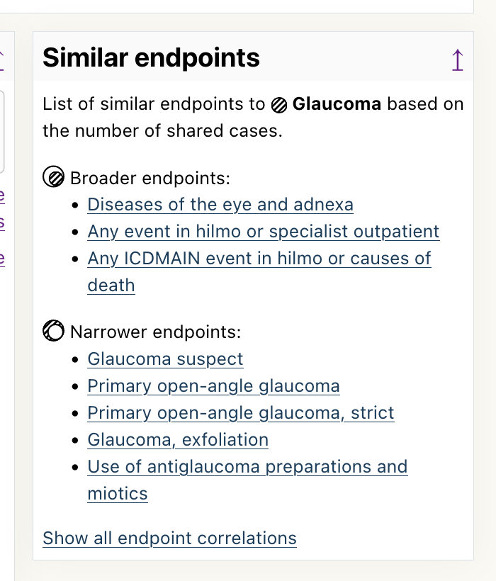
2. Locate the Similar endpoints box near the top of the page.

3. Related endpoints which are a strict superset of cases of the current endpoint are shown in Broader endpoints, and endpoints which are a strict subset of cases are shown in Narrower endpoints.

   

Using the Correlations table

1. Go to the endpoint page of your endpoint of interest.
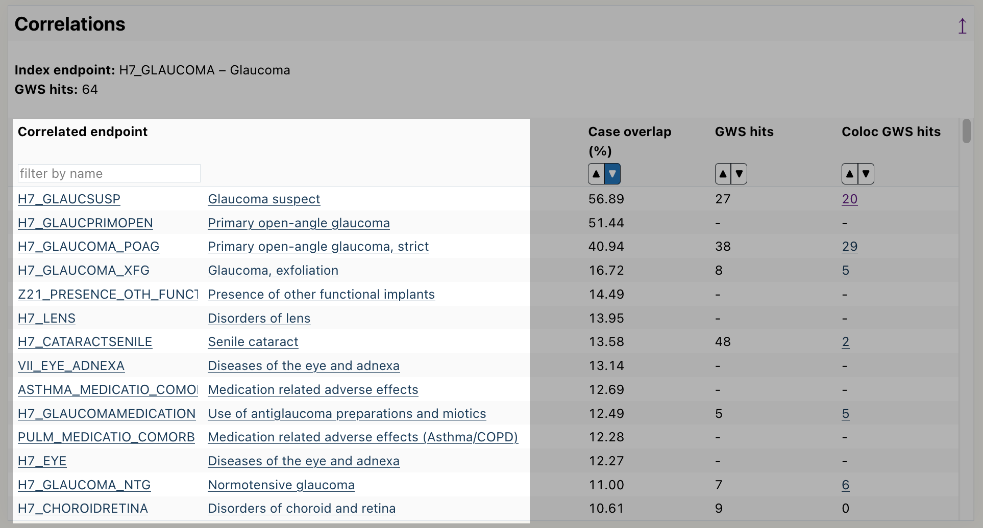
2. Scroll down to the correlation table.

3. Read the endpoints from the table, by default it is sorted by highest case overlap between endpoints.

   

How to get more detailed data on an endpoint? (e.g. data for N<5, histograms with narrower bins)

Risteys doesn't provide data where any data point has less than 5 individuals.

More detailed data is available in the FinnGen sandbox. See the FinnGen Analyst Handbook documentation.

How to get measurements that are not shown in Risteys? (e.g. BMI, ECG)

Risteys doesn't provide such measurements at the moment.

It is worth looking in the FinnGen Analyst Handbook if such measurements are available through other means.

Where does the data come from?

The data in Risteys comes from FinnGen. Different Finnish health registries make up the phenotypic data of FinnGen, which in turn is used to build Risteys.

The main registries used in Risteys are:

• Care Register for Health Care (HILMO)
• Population registry (DVV)
• Cause of death
• Finnish Cancer Registry
• Drug purchase and reimbursement (Kela)

Have a look at Finnish health registries page of the FinnGen Analyst Handbook for detailed information.

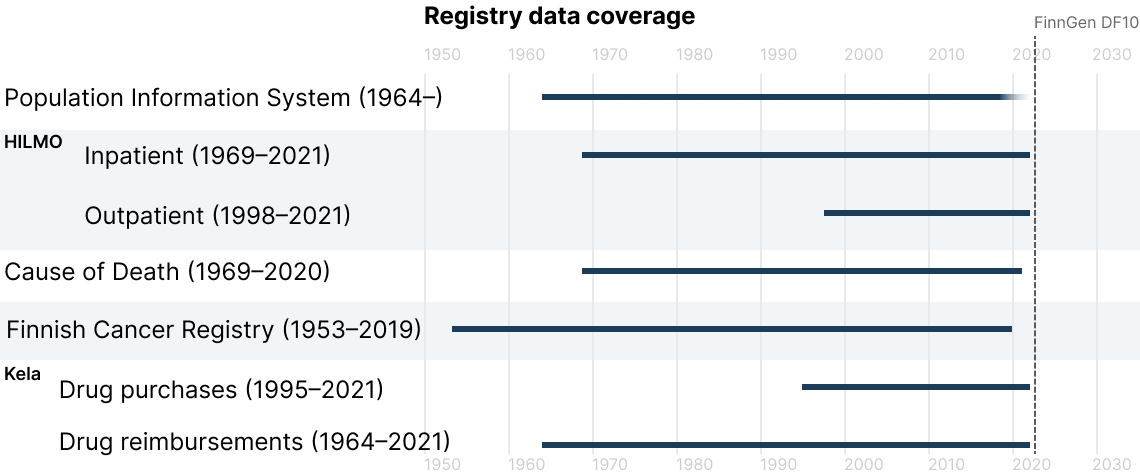
Which years are covered by the different health registries?

The registries used in Risteys vary in their coverage of the data. This image shows which years are covered by each registry:

What is the difference between ICD-10 and ICD-10-fi?

Many places in FinnGen reference ICD-10 and sometimes ICD-10-fi. Both are similar classifications used in electronic health records, they map codes to health conditions.

ICD-10-fi is a variant of ICD-10 introduced by the Finnish health care system.

The main differences between ICD-10 and ICD-10-fi are:

• Some codes are only in ICD-10, while some codes are only in ICD-10-fi. Though most of the codes are shared between ICD-10 and ICD-10-fi.
• ICD-10-fi as definitions for combining symptom and cause into a single code. For example: A01.1 Typhoid fever as cause and G01 Meningitis as symptom is the single code A01.1+G01 Meningitis associated with typhoid fever in ICD-10-fi.
• ICD-10-fi has a notation to indicate causal medication.

Why is an endpoint defined with ICD-10 but no ICD-9 no ICD-8?

The two main reasons are:

• The people that defined the endpoint knew which ICD-10 to pick when creating the endpoint, but they didn't know if any ICD-9 or ICD-8 could also be used.
• The people that defined the endpoint know there is no corresponding ICD-9 or 8 that could be used. This is indicated with the symbol $!$.

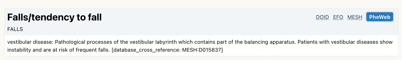
Why are some endpoint descriptions wrong?

In some cases the description shown below the endpoint page will be wrong, like in this example:

This happens because the descriptions are not written as part of FinnGen. Instead they are gathered from various sources, and we try to programmatically attribute the best description to all the FinnGen endpoints. But sometimes our algorithm fails.

Methods

• Key figures & distributions
• Cumulative incidence function (CIF)
• Mortality

Key figures & distributions

The key figures include the following statistics:

• Number of individuals: Number of individuals with the endpoint of interest
• Unadjusted prevalence: Number of individuals with the endpoint of interest divided by the total number of individuals in FinnGen
• Mean age at first event: Mean age at the first occurrence of the endpoint

Distributions are presented by age and year at the first event. Bars in distributions are aggregated to include at least 5 individuals.

Mortality

The goal of the analysis is to calculate the association between an exposure endpoint and death.

Data pre-processing

• Start of follow-up: 1998-01-01 – we choose this date because we have complete coverage for all registries
• End of follow-up: death or 2021-12-31
• If the date of diagnoses for the exposure endpoint happens before 1998-01-01 we assume that it happened on 1998-01-01.
• Only calculated if there are at least 10 deaths among individuals diagnosed with the exposure endpoint

Case-cohort design

To improve computational speed, we used a case-cohort design.

Briefly, from the original cohort, we selected a subcohort at the start of follow-up. The subcohort can include individuals that died. The size of the subcohort is 10,000 individuals. The final population includes all the individuals in the subcohort and all the individuals that died outside the subcohort.

Cox regression

To perform the analyses, we used a Cox regression with a time-varying covariate, weighted by the inverse of the sampling probability to account for the case-cohort design. Robust standard error was used. The model is defined as:
Surv(time,death) ~ exposure_endpoint + birth_year + sex

• time is calculated as (date end of follow-up – date entry in the study) as defined in Data pre-processing (except for individuals diagnosed with the exposure endpoint where time is split from entry till diagnosis and from diagnosis till the end of follow up, see below).
• exposure_endpoint is treated as a time-varying covariate. This means that an individual is unexposed (value of the variable is set to 0) from 1998-01-01 until the diagnoses of the exposure endpoint and exposed (value of the variable is set to 1) after that. That is, if an individual experiences an exposure endpoint, it will have two rows in the dataset.

Lagged hazard ratios are computed with the following follow-up time windows: < 1 year, between 1 and 5 years, between 5 and 15 years.

The Cox regression is implemented using the lifelines library.

Absolute Risk (AR)

The absolute risk represents the probability of dying. It is defined as AR = 1 - survival_probability. The survival probability is derived using the Breslow’s method assuming these values for the other covariates in the model:

• year of birth: 1959
• sex ratio: 50%

Survival analyses between endpoints

Associations between endpoints are calculated loosely following the approach described in the NB-COMO study. The goal of the analysis is to study the association between an exposure endpoint and an outcome endpoint. E.g., what’s the association between a diagnosis of type 2 diabetes (exposure endpoint) and cardiovascular diseases (outcome endpoint).

Data pre-processing

• Start of follow-up: 1998-01-01 – we choose this date because we have complete coverage for all registries
• End of follow-up: diagnose of the outcome endpoint or death or 2021-12-31
• Prevalent cases (i.e. individuals that have been diagnosed with the outcome endpoint before 1998-01-01) were removed from the study. We consider only incident cases.
• If the date of diagnoses for the exposure endpoint happens before 1998-01-01 we assume that it happened on 1998-01-01.
• Only consider endpoint pairs:
  • with at least 10 individuals for each cell of the 2x2 contingency table between endpoint pairs.
  • with at least 25 individuals having the outcome endpoint.
  • where endpoints are not “overlapping”. That is, endpoints are not descendants of one another endpoint in the tree hierarchy or have overlapping underlying ICD codes.

Case-cohort design

To improve computational speed, we used a case-cohort design.

Briefly, from the original cohort, we selected a subcohort at the start of follow-up. The subcohort can include outcome endpoints. The size of the subcohort is always 10,000 individuals randomly selected for each analysis. The final population includes all the individuals in the subcohort and all the individuals that experience the outcome endpoints outside the subcohort.

Cox regression

To perform the analyses, we used a Cox regression with a time-varying covariate, weighted by the inverse of the sampling probability to account for the case-cohort design. Robust standard error was used. The model is defined as:
Surv(time,outcome_endpoint) ~ exposure_endpoint + birth_year + sex

• time is calculated as (date end of follow-up – date entry in the study) as defined in Data pre-processing (except for individuals diagnosed with the exposure endpoint where time is split from entry till diagnosis and from diagnosis till the end of follow up, see below).
• exposure_endpoint is treated as a time-varying covariate. This means that an individual is unexposed (value of the variable is set to 0) from 1998-01-01 until the diagnoses of the exposure endpoint and exposed (value of the variable is set to 1) after that. That is, if an individual experiences an exposure endpoint, it will have two rows in the dataset.

Lagged hazard ratios are computed with the following follow-up time windows: < 1 year, between 1 and 5 years, between 5 and 15 years. If an outcome endpoint happens outside the time-widow, the individual experience the disease is kept, but the outcome endpoint is not considered (i.e. variable is set to 0).

The Cox regression is implemented using the lifelines library.

Drug Statistics

The drug score is computed in a 2-step process:

1. Fit the data to the logistic model:
   y ~ sex + year-of-birth + year-of-birth^2 + year-at-endpoint + year-at-endpoint^2
   
2. Use the fitted model to predict the probability for the following data:
   • sex = 0.5, assume an even number of females and males.
   • year-of-birth = 1960, the mean year of birth of the FinnGen cohort.
   • year-at-endpoint = 2021, predict the probability at the end of the study.

The resulting probability value is the drug score. The highest the drug score is, the more likely the drug is to be taken after the given endpoint.

Notes

Due to the sensitive nature of the data, the age when entering and leaving the study has an accuracy of 1 year.